cvCovEst: Cross-Validated
Covariance Matrix Estimation
Philippe Boileau, Brian Collica, Nima Hejazi
2022-12-07
Source:vignettes/using_cvCovEst.Rmd
using_cvCovEst.RmdBackground and Motivation
When the number of observations in a dataset far exceeds the number of features, the estimator of choice for the covariance matrix is the sample covariance matrix. It is an efficient estimator under minimal regularity assumptions on the data-generating distribution. In high-dimensional regimes, however, this estimator leaves much to be desired: The sample covariance matrix is either singular, numerically unstable, or both, thereby amplifying estimation error.
As high-dimensional data have become widespread, researchers have derived many novel covariance matrix estimators to remediate the sample covariance matrix’s deficiencies. These estimators come in many flavours, though most are constructed by regularizing the sample covariance matrix, or through the estimation of latent factors. A comprehensive review is provided by Fan, Liao, and Liu (2016).
This variety brings with it many challenges. Identifying an “optimal” estimator from among a collection of candidates can prove a daunting task, one whose objectivity is often compromised by the analyst’s decisions. Though data-driven approaches for selecting an optimal estimator from among estimators belonging to certain (limited) classes have been derived, the question of selecting an estimator from among a diverse collection of candidates remains unaddressed.
We therefore offer a general, cross-validation-based framework for covariance matrix estimator selection to tackle just that. The high-dimensional asymptotic optimality of selections are guaranteed based upon extensions of the seminal work of Dudoit and van der Laan (2003), Dudoit and van der Laan (2005), and van der Vaart, Dudoit, and van der Laan (2006) on data-adaptive estimator selection to high-dimensional covariance matrix estimation (Boileau et al. 2021). The interested reader is invited to review theoretical underpinnings of the methodology as described in Boileau et al. (2021).
Cross-validated Covariance Matrix Estimation
Let there be a high-dimensional dataset comprising \(n\) realizations of \(i.i.d.\) \(p\)-length random vectors with a possibly nonparametric data-generating distribution. Our goal is to estimate these random vectors’ covariance matrix, which may be accomplished using our general cross-validated estimator selection framework.
Given a library of candidate estimators, a loss function, and a
choice of cross-validation scheme, cvCovEst() will identify
the asymptotically optimal estimator of the covariance matrix from among
all candidates. It subsequently estimates this parameter using the
selected candidate. An example is provided below. Lists and brief
descriptions of implemented candidate estimators, loss functions, and
cross-validation schemes are provided in the sequel.
## Warning: package 'MASS' was built under R version 4.1.2## cvCovEst v1.2.0: Cross-Validated Covariance Matrix Estimation
set.seed(1584)

# generate a 50x50 covariance matrix with unit variances and off-diagonal
# elements equal to 0.5
sigma <- matrix(0.5, nrow = 50, ncol = 50) + diag(0.5, nrow = 50)

# sample 50 observations from multivariate normal with mean = 0, var = Sigma
dat <- mvrnorm(n = 50, mu = rep(0, 50), Sigma = sigma)

# run CV-selector
cv_cov_est_out <- cvCovEst(
    dat = dat,
    estimators = c(
      linearShrinkLWEst, denseLinearShrinkEst,
      thresholdingEst, poetEst, sampleCovEst
    ),
    estimator_params = list(
      thresholdingEst = list(gamma = c(0.2, 0.4)),
      poetEst = list(lambda = c(0.1, 0.2), k = c(1L, 2L))
    ),
    cv_loss = cvMatrixFrobeniusLoss,
    cv_scheme = "v_fold",
    v_folds = 5,
  )

# print the table of risk estimates
cv_cov_est_out$risk_df
## # A tibble: 9 × 3
## estimator hyperparameters cv_risk
## <chr> <chr> <dbl>
## 1 linearShrinkLWEst hyperparameters = NA 357.
## 2 poetEst lambda = 0.2, k = 1 369.
## 3 poetEst lambda = 0.2, k = 2 372.
## 4 poetEst lambda = 0.1, k = 2 375.
## 5 poetEst lambda = 0.1, k = 1 376.
## 6 denseLinearShrinkEst hyperparameters = NA 379.
## 7 sampleCovEst hyperparameters = NA 379.
## 8 thresholdingEst gamma = 0.2 384.
## 9 thresholdingEst gamma = 0.4 505.
# print a subset of the selected estimator's estimate
cv_cov_est_out$estimate[1:5, 1:5]
## [,1] [,2] [,3] [,4] [,5]
## [1,] 1.1725637 0.5219385 0.4813226 0.5576840 0.6719526
## [2,] 0.5219385 0.9364171 0.5591108 0.4390799 0.6766744
## [3,] 0.4813226 0.5591108 1.0150440 0.4052703 0.6436765
## [4,] 0.5576840 0.4390799 0.4052703 0.9826984 0.4304168
## [5,] 0.6719526 0.6766744 0.6436765 0.4304168 1.0883278Candidate Estimators
Covariance matrix estimators implemented in the cvCovEst
package are catalogued in the following table. These estimators are fed
to the cvCovEst() function through the
estimators argument as a vector. If these estimators rely
on hyperparameters, then they must be passed to the
estimator_params as a list. Depending on one’s assumptions
— or lack thereof — about the true covariance matrix, one may choose to
use a subset of these estimators or all of them. Of course, they may
also be used as standalone functions.
| Estimator | Implementation | Description |
|---|---|---|
| Sample covariance matrix | sampleCovEst() |
The sample covariance matrix. |
| Hard thresholding (Bickel and Levina 2008b) | thresholdingEst() |
Applies a hard thresholding operator to the entries of the sample covariance matrix. |
| SCAD thresholding (Rothman, Levina, and Zhu 2009; Fan and Li 2001) | scadEst() |
Applies the SCAD thresholding operator to the entries of the sample covariance matrix. |
| Adaptive LASSO (Rothman, Levina, and Zhu 2009) | adaptiveLassoEst() |
Applies the adaptive LASSO thresholding operator to the entries of the sample covariance matrix. |
| Banding (Bickel and Levina 2008a) | bandingEst() |
Replaces the sample covariance matrix’s off-diagonal bands by zeros. |
| Tapering (Cai, Zhang, and Zhou 2010) | taperingEst() |
Tapers the sample covariance matrix’s off-diagonal bands, eventually replacing them by zeros. |
| Optimal Linear Shrinkage (Ledoit and Wolf 2004) | linearShrinkLWEst() |
Asymptotically optimal shrinkage of the sample covariance matrix towards the identity. |
| Linear Shrinkage (Ledoit and Wolf 2004) | linearShrinkEst() |
Shrinkage of the sample covariance matrix towards the identity, but the shrinkage is controlled by a hyperparameter. |
| Dense Linear Shrinkage (Schäfer and Strimmer 2005) | denseLinearShrinkEst() |
Asymptotically optimal shrinkage of the sample covariance matrix towards a dense matrix whose diagonal elements are the mean of the sample covariance matrix’s diagonal, and whose off-diagonal elements are the mean of the sample covariance matrix’s off-diagonal elements. |
| Nonlinear Shrinkage (Ledoit and Wolf 2018) | nlShrinkLWEst() |
Analytical estimator for the nonlinear shrinkage of the sample covariance matrix. |
| POET (Fan, Liao, and Mincheva 2013) | poetEst() |
An estimator based on latent variable estimation and thresholding. |
| Robust POET (Fan, Liu, and Wang 2018) | robustPoetEst() |
A robust (and more computationally taxing) take on the POET estimator. |
| Spiked Operator Loss Shrinkage (Donoho, Gavish, and Johnstone 2018) | spikedOperatorShrinkEst() |
The asymptotically optimal shrinkage estimator based on the operator loss in a Gaussian spiked covariance model. |
| Spiked Frobenius Loss Shrinkage (Donoho, Gavish, and Johnstone 2018) | spikedFrobeniusShrinkEst() |
The asymptotically optimal shrinkage estimator based on the Frobenius loss in a Gaussian spiked covariance model. |
| Spiked Stein Loss Shrinkage (Donoho, Gavish, and Johnstone 2018) | spikedSteinShrinkEst() |
The asymptotically optimal shrinkage estimator based on the Stein loss in a Gaussian spiked covariance model. |
Note that cvCovEst() only functions with estimators
native to this package. If you’d like to request a new estimator
implementation, please submit an issue to the
queue.
Loss Functions
Given a collection of candidate estimators, cvCovEst()
compares their conditional cross-validated risks to identify the optimal
selection. The loss function used to compute these risks should reflect
both aspects of the data-generating distribution and the goal of the
estimation procedure. This package currently implements three loss
functions:
| Loss | Implementation | Description |
|---|---|---|
| Matrix-based Frobenius | cvMatrixFrobeniusLoss() |
The default, based on the Frobenius norm. Appropriate when the dataset’s features are of similar magnitudes. |
| Variance-scaled matrix-based Frobenius | cvScaledMatrixFrobeniusLoss() |
A scaled version of the matrix-based Frobenius loss, where weights are the inverse of products from the sample covariance matrix’s diagonal. Appropriate when the features of the dataset are of different magnitudes. |
| Observation-based Frobenius | cvFrobeniusLoss() |
Based on the Frobenius norm and the rank-1, observation-level estimates of the sample covariance matrix. Its selections are equivalent to that of the matrix-based Frobenius, though less computationally efficient. However, the optimality results of Boileau et al. (2021) rely on it. |
The choice of loss function is set trough the cv_loss
argument. Like the candidate estimators, cvCovEst() only
supports loss functions implemented in this package. Please submit
suggestions to the issue
queue.
Supported Cross-Validation Schemes
Two cross-validation schemes are currently supported by
cvCovEst(). Please consider filing an issue in the
queue to request the implementation of another cross-validation
scheme.
| Scheme | Details |
|---|---|
| V-fold | To use V-fold cross-validation, set the cv_scheme
argument in cvCovEst() to "v_fold", and set
the number of folds through the v_folds argument.
cvCovEst() defaults to 5-fold cross-validation. |
| Monte-Carlo | To perform Monte-Carlo cross-validation, set the
cv_scheme argument to "mc". Set the proportion
of data to be used in each validation set using the
mc_split argument, and the number of iterations to perform
with the v_folds argument. |
Diagnostic Tools
In addition to selecting an optimal estimator, the
cvCovEst package contains summary and plotting methods
which highlight the statistical properties of the candidate estimators,
and inform the performance of the selection framework. These tools help
build intuition about these estimators’ behavior and allows for the
evaluation of their performance over varying inputs.
Summary Method
The summary() method for cvCovEst accepts
an object argument, a named list of class
cvCovEst, a dat_orig argument, the original
data used to calculate the covariance matrix estimates, and a
summ_fun argument, a character vector specifying the type
of summary function to use.
These summary functions allow the user to quickly compare the
performance of several classes of estimators and compute other metrics
of interest. The choices of summ_fun and their outputs are
described below:
| Summary | Implementation | Description |
|---|---|---|
| Empirical Risk by Estimator Class | empRiskByClass |
Returns the minimum, 1st quartile, median, 3rd
quartile, and maximum of the empirical risk associated with each class
of estimator passed to cvCovEst(). |
| Best Performing Estimator by Class | bestInClass |
Returns the specific hyperparameters, if applicable, of the best performing estimator within each class along with additional metrics. |
| Worst Performing Estimator by Class | worstInClass |
Returns the specific hyperparameters, if applicable, of the worst performing estimator within each class along with additional metrics. |
| Empirical Risk by Hyperparameter | hyperRisk |
For estimators that take hyperparameters as arguments, this returns
the hyperparameters associated with the minimum, 1st
quartile, median, 3rd quartile, and maximum of the empirical
risk within each class of estimator. Each class has its own
tibble which are returned as a list. |
When either bestInClass or worstInClass is
specified, the additional metrics are the condition number, the sign,
and the sparsity. Sign refers to the estimate’s sign and is one of
positive-definite ("PD"), positive-semi-definite (“PSD”),
negative-definite (“ND”), negative-semi-definite (“NSD”), or indefinite
(“IND”). If an estimate results in a zero matrix, then the sign is
returned as "NA". Sparsity is calculated at the proportion
of total entries in the estimate which are equal to zero.
Plot Method
The plot() method for cvCovEst allows users
to visualize three main plot_types of the candidate
estimators: covariance heat maps (heatmap), eigenvalue
plots (eigen), and the empirical risk (risk)
as a function of the hyperparameters (for applicable estimator classes).
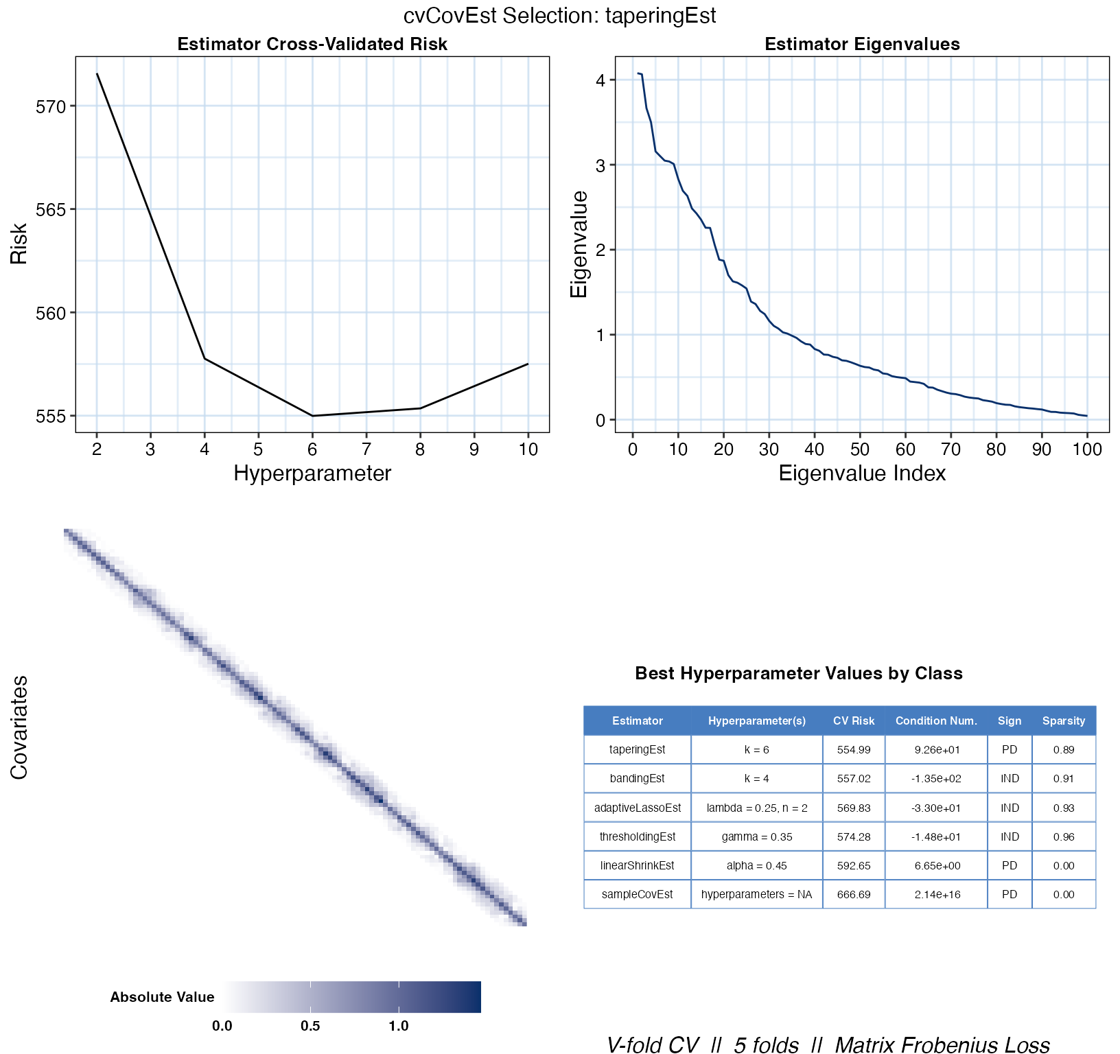
If users do not specify a plot type, then all three plots are combined
into one figure for the optimal estimator selected by
cvCovEst(). Users can also achieve this by setting
plot_type = "summary".
The heat maps and eigenvalue plots facilitate comparisons both within
and between estimator classes by allowing multiple values to be passed
as estimator and stat arguments.
Additional arguments specific to each plot_type are
outlined below:
Heat Map
| Argument | Description |
|---|---|
| abs_v | If TRUE, then the absolute value of the covariance is
mapped. Otherwise, the signed value is used. |
Eigenvalue Plot
| Argument | Description |
|---|---|
| leading | If TRUE, then the k leading eigenvalues are displayed.
Otherwise, the k trailing eigenvalues are displayed. |
| k | The number of leading or trailing eigenvalues to plot. |
Empirical Risk
These two additional arguments only apply to estimators with multiple hyperparameters:
| Argument | Description |
|---|---|
| switch_vars | If TRUE, the hyperparameters used for the x-axis and
factor variables are switched. |
| min_max | If TRUE, only the minimum and maximum values of the
factor hyperparameter will be used. |
Simulated Data Analysis Example
To show how the plot and summary methods can be used, data is
simulated from a predetermined covariance matrix following a Toeplitz
structure. The data is then passed to cvCovEst() along with
a handful of estimators.
set.seed(1584)

toep_sim <- function(p, rho, alpha) {
    times <- seq_len(p)
    H <- abs(outer(times, times, "-")) + diag(p)
    H <- H^-(1 + alpha) * rho
    covmat <- H + diag(p) * (1 - rho)

    sign_mat <- sapply(
      times,
      function(i) {
        sapply(
          times,
          function(j) {
            (-1)^(abs(i - j))
          }
        )
      }
    )
    return(covmat * sign_mat)
}

# simulate a 100 x 100 covariance matrix
sim_covmat <- toep_sim(p = 100, rho = 0.6, alpha = 0.3)

# sample 75 observations from multivariate normal mean = 0, var = sim_covmat
sim_dat <-  MASS::mvrnorm(n = 100, mu = rep(0, 100), Sigma = sim_covmat)

# run CV-selector
cv_cov_est_sim <- cvCovEst(
  dat = sim_dat,
  estimators = c(
    linearShrinkEst, thresholdingEst, bandingEst, adaptiveLassoEst,
    sampleCovEst, taperingEst
  ),
  estimator_params = list(
    linearShrinkEst = list(alpha = seq(0.25, 0.75, 0.05)),
    thresholdingEst = list(gamma = seq(0.25, 0.75, 0.05)),
    bandingEst = list(k = seq(2L, 10L, 2L)),
    adaptiveLassoEst = list(lambda = c(0.1, 0.25, 0.5, 0.75, 1), n = seq(1, 5)),
    taperingEst = list(k = seq(2L, 10L, 2L))
  ),
  cv_scheme = "v_fold",
  v_folds = 5
)
Summary Method
The summary() method is then used to compare the best
performing estimators in each class:
cv_sum <- summary(cv_cov_est_sim, dat_orig = sim_dat)
cv_sum$bestInClass
## # A tibble: 6 × 6
## estimator hyperparameter cv_risk cond_num sign sparsity
## <chr> <chr> <dbl> <dbl> <chr> <dbl>
## 1 taperingEst k = 6 555. 9.26e 1 PD 0.89
## 2 bandingEst k = 4 557. -1.35e 2 IND 0.91
## 3 adaptiveLassoEst lambda = 0.25, n = 2 570. -3.3 e 1 IND 0.93
## 4 thresholdingEst gamma = 0.35 574. -1.48e 1 IND 0.96
## 5 linearShrinkEst alpha = 0.45 593. 6.65e 0 PD 0
## 6 sampleCovEst hyperparameters = NA 667. 2.14e16 PD 0In this case, the tapering estimator with k = 6 achieves
the lowest empirical risk. It is also one of the few positive definite
matrices, though its condition number is worse than that of the linear
shrinkage estimator’s estimate. The resulting estimate is also less
sparse than that of the other sparsity-enforcing estimators “best”
estimates.
We can take a closer look at the estimator’s performance based on
other possible hyperparameter values by hashing taperingEst
from the hyperRisk list.
cv_sum$hyperRisk$taperingEst## # A tibble: 5 × 3
## hyperparameters cv_risk stat
## <chr> <chr> <chr>
## 1 k = 6 555 min
## 2 k = 6 555 Q1
## 3 k = 6 555 median
## 4 k = 4 558 Q3
## 5 k = 2 572 maxPlot Method
By specifying plot_type = "risk", we can see the change
in empirical risk as the value of k changes. A summary of
the cross-validation scheme and loss function is displayed at the bottom
of all cvCovEst plot outputs.
plot(cv_cov_est_sim, dat_orig = sim_dat, plot_type = "risk")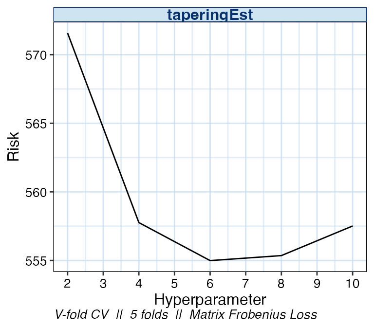
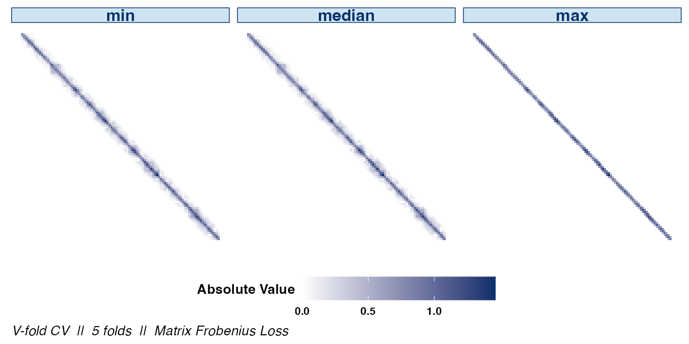
We can also examine the matrix structure as the value of
k changes. Examining the overall sparsity of the resulting
estimator can be useful since, in some cases, the assumption of sparsity
is not warranted. Note that the absolute values of the estimate’s
entries are displayed to emphasize the structural differences between
choices of hyperparameters.
If the signs of the covariances are of interest, they can be
displayed by setting abs_v = FALSE:
plot(cv_cov_est_sim, dat_orig = sim_dat, plot_type = "heatmap",
     stat = c("min", "median", "max"), abs_v = FALSE)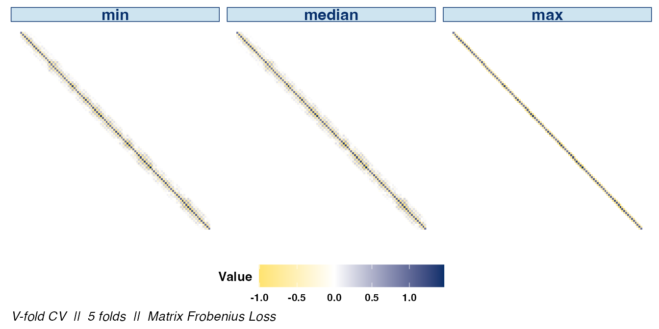
The difference between the optimal estimator selected by
cvCovEst() and the sample covariance matrix is clear when
displaying their respective heat maps side by side.
plot(cv_cov_est_sim, dat_orig = sim_dat, plot_type = "heatmap",
     estimator = c("taperingEst", "sampleCovEst"),
     stat = c("min"), abs_v = FALSE)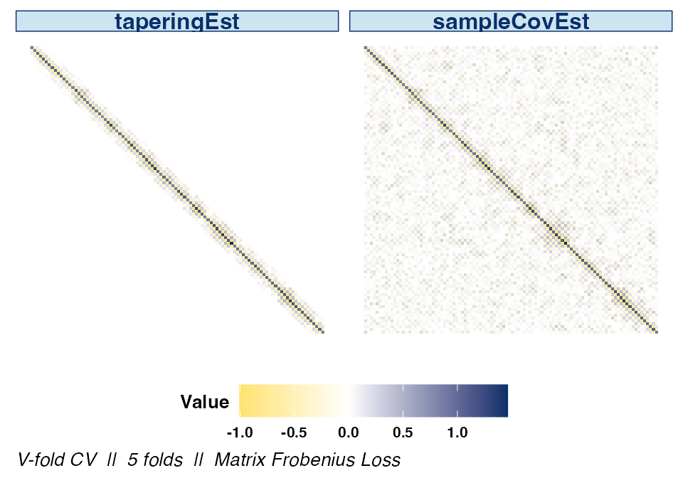
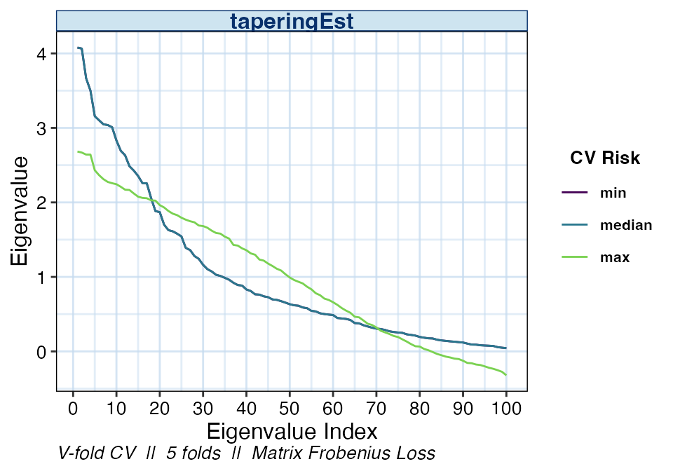
We may also be interested in the eigenvalues of the various banding
estimators. The distribution of eigenvalues relays information such as
the condition number or the positive-definiteness of the resulting
estimator. As with the other plot types, if the estimator
argument is not specified, the default is to display the optimal
estimator selected by cvCovEst().
Specifying multiple values in the estimator argument
allows us compare the eigenvalues of the other estimator classes as
well.
plot(cv_cov_est_sim, dat_orig = sim_dat, plot_type = "eigen",
     stat = c("min", "median", "max"),
     estimator = c("taperingEst", "bandingEst", "linearShrinkEst",
                    "adaptiveLassoEst"))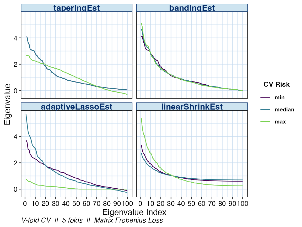
As previously mentioned, simply calling the plot() on
the output of cvCovEst() and providing the original data
will result in a visual summary of the selected estimator.
plot(cv_cov_est_sim, dat_orig = sim_dat)